DBSCAN Tuning
DBSCAN’s accuracy and performance can be improved by tuning its hyperparameters. Here is a list with some optimization tricks that can improve the results you’re getting from DBSCAN implementations
Limiting feature amount in the splits
1- eps
This parameter is used to check the neighbor relation between samples and it is a major criteria for clustering in DBSCAN. If a sample doesn’t have enough (min_samples) samples within a range of eps in its proximity it won’t be clustered and it will remain an outlier.
So, for each sample point, DBSCAN checks other samples in eps range from it. There needs to be minimum amount ( (see next parameter) of neighbors in that scan for the sample point to belong to that cluster.
eps is 5 by default in the Scikit-Learn DBSCAN implementation. You can change it to another value simply by using the eps parameter.
Here is an example to adjust eps value in Python:
DBS = DBSCAN(eps = 1)
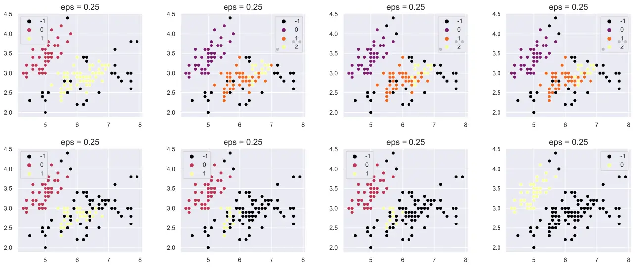
In this case eps value will be set to 1 meaning in a distance of 1 DBSCAN will scan for neighbors. It will be more inclusive compared to eps=0.5 and some outlier values who would be left out might get included in clusters.
Increase in eps is also likely to result in less clusters overall after DBSCAN algorithm finishes running.
DBSCAN eps
- negative correlation with cluster amount
- negative correlation with outlier amount
- default, 0.5
DBSCAN min_samples
- criterion
- splitter
- default, 5
Limiting feature amount in the splits
2- min_samples
This parameter works in tandem with eps parameter. DBSCAN will iterate each sample point and look for min_samples amount of neighbors in a distance of eps from the sample point. If there aren’t min_samples amount of neighbors in range, sample will be labeled as an outlier.
Here is a Python code example:
DBS = DBSCAN(eps = 1)
Limiting feature amount in the splits
3- metric and p
metric parameter is used to define the metric used in distance calculations between samples in DBSCAN algorithm. There are a number of metrics that can be used such as “euclidean” “manhattan” or “minkowski”. If you use “minkowski” metric you can also use p parameter to define the power of minkowski metric.
You can see a Python code for a set of minkowski metric and a p value of 2 below:
DBS = DBSCAN(metric = "minkowski", p=2)
Limiting feature amount in the splits
4- algorithm
This parameter defines the algorithm used for distance calculations. There are 3 options but a 4th option: “auto” is successfully utilized in the Scikit-Learn implementation of DBSCAN algorithm. 3 algorithm options are:
- brute : Each point will be mapped and vectorized prior to distance calculations.
- kd_tree : Data will be mapped as a tree structure improving the runtime and complexity.
- ball_tree : Also creates a tree structure to map and vectorize the samples in the dataset.
The difference between kd_tree and ball_tree is the way they structure trees to organize and vectorize data. kd_tree is a binary tree algorithm that splits data in two and then continues splitting the splits by two and so on until it ends up with a minimum leaf size.
Ball_tree algorithm does what kd_tree algorithm does but it uses centroids to build a binary tree structure, hence the name ball, until it ends up with the minimum leaf size. Depending on the dataset’s order, size, dimensions and other characteristics sometimes ball_tree will have the upper hand compared to the kd_tree algorithm but kd_tree is slightly more utilized in general.
Leaf node is the end node in a tree structure and it includes a number of sample points. When kd_tree or ball_tree are utilized, leaf_size parameter can also be adjusted which is the next parameter in the list.
DBS = DBSCAN(eps = 1)
kd_tree
- binary tree algorithm
- splits data in half based on values
- suitable for large datasets
ball_tree
- binary tree algorithm
- splits data in half based on centroids
- suitable for large datasets
Limiting feature amount in the splits
5- leaf_size
This parameter is used when algorithm parameter is set to kd_tree or ball_tree. It defines the size of the leaf_node and it has implications on the way data is handled.
By default leaf_size is 30. If you increase leaf_size data will be processed in larger chunks but this may increase the likelihood of wrong neighbors ending up in the wrong batch which may be less ideal depending on the data.
On the other hand, increasing leaf_size might mean improved performance. The opposite case of increased leaf_size is decreased leaf_size. For example leaf_size=1 will equal the brute_force algorithm which means each sample is handled one by one resulting in a potentially increased accuracy but decreased performance and use of computation resources.
DBS = DBSCAN(algorithm = "kd_tree", leaf_size=500)
Limiting feature amount in the splits
6- n_jobs
This parameter can be very useful to improve the performance of DBSCAN algorithm and make it faster. n_jobs is used to parallelize DBSCAN computation. It is 1 by default meaning there is no parallelization being utilized but you can set this value to the amount of cores in the processor.
A common application is also to set it to -1 which will parallelize all the cores making most use of parallel computation and improve the runtime as much as possible.
It can be adjusted simply by a Python code as below:
DBS = DBSCAN(n_jobs = -1)
Summary
In this DBSCAN Tutorial, we’ve seen the most commonly used DBSCAN parameters that can be used to improve performance and accuracy.
Being familiar with these DBSCAN parameters and knowing how to optimize them can help greatly to achieve better machine learning results and acquire game-changing insight from large and complex datasets.